Initial Conditions#
Currently we provide the following initial conditions:
Initial Conditions via Easi#
You can input your initial conditions via an easi file. For that, set
&IniCondition
cICType = 'easi'
filename = '$INIFILE'
hastime = 1
Then, input the initial condition into the easi file $INIFILE. For the variable names, use the same as used in the output.
For example, for elastic (and viscoelastic etc.), a (rather nonsensical) constant initial condition looks as follows:
!ConstantMap
map:
  s_xx: 1
  s_yy: 4
  s_zz: 9
  s_xy: 16
  s_xz: 25
  s_yz: 36
  v1: 49
  v2: 64
  v3: 81
Of course, one may use Lua functions or ASAGI as input as well for several variables.
The parameter hastime indicates that the easi file has t as a time input variable besides the spatial coordinates (x,y,z).
This way, the easi boundary condition can be used for comparing against after time has passed (e.g. for convergence tests).
However, it requires easi 1.5.0 or higher to function correctly.
As a caveat, the Easi initial condition currently does not support the analytical boundary condition.
Hard-Coded Initial Conditions#
Since the old days, some initial conditions were hard coded into SeisSol. To select these, it suffices to set
&IniCondition
cICType = '$NAME'
where $NAME is the name of one of the following inital conditions.
Zero (Zero)#
All quantities are set to zero. This is the standard case to work with point sources or dynamic rupture.
Planar wave (Planarwave)#
A planar wave for convergence tests. The inital values are computed such that a planar wave in a unit cube is imposed. For elastic, anisotropic and viscoelastic materials, we impose a P and an S wave travelling in opposite directions. For poroelastic materials, we impose a slow P and an S wave travelling in one direction and a fast P wave travelling in opposite direction. This scenario needs periodic boundary conditions to make sense. This is the only case where the old netcdf mesh format is prefered. After the simulation is finished the errors between the analytic solution and the numerical one are plotted in the \(L^1\)-, \(L^2\)- and \(L^\infty\)-norm.
You can use the cubegenerator mesh type to make SeisSol generate meshes for
convergence tests.
Alternatively, use cube_c to do so:
SeisSol/SeisSol
Superimposed planar wave (SuperimposedPlanarwave)#
Superimposed three planar waves travelling in different directions. This is especially interesting in the case of directional dependent properties such as for anisotropic materials.
Travelling wave (Travelling)#
Impose one period of a sinusoidal planar wave as initial condition, see for example the video below. There, we impose a P wave travelling to the left. The wave speed at the top and bottom is \(2 m/s\) and \(2.83 m/s\) in the middle.
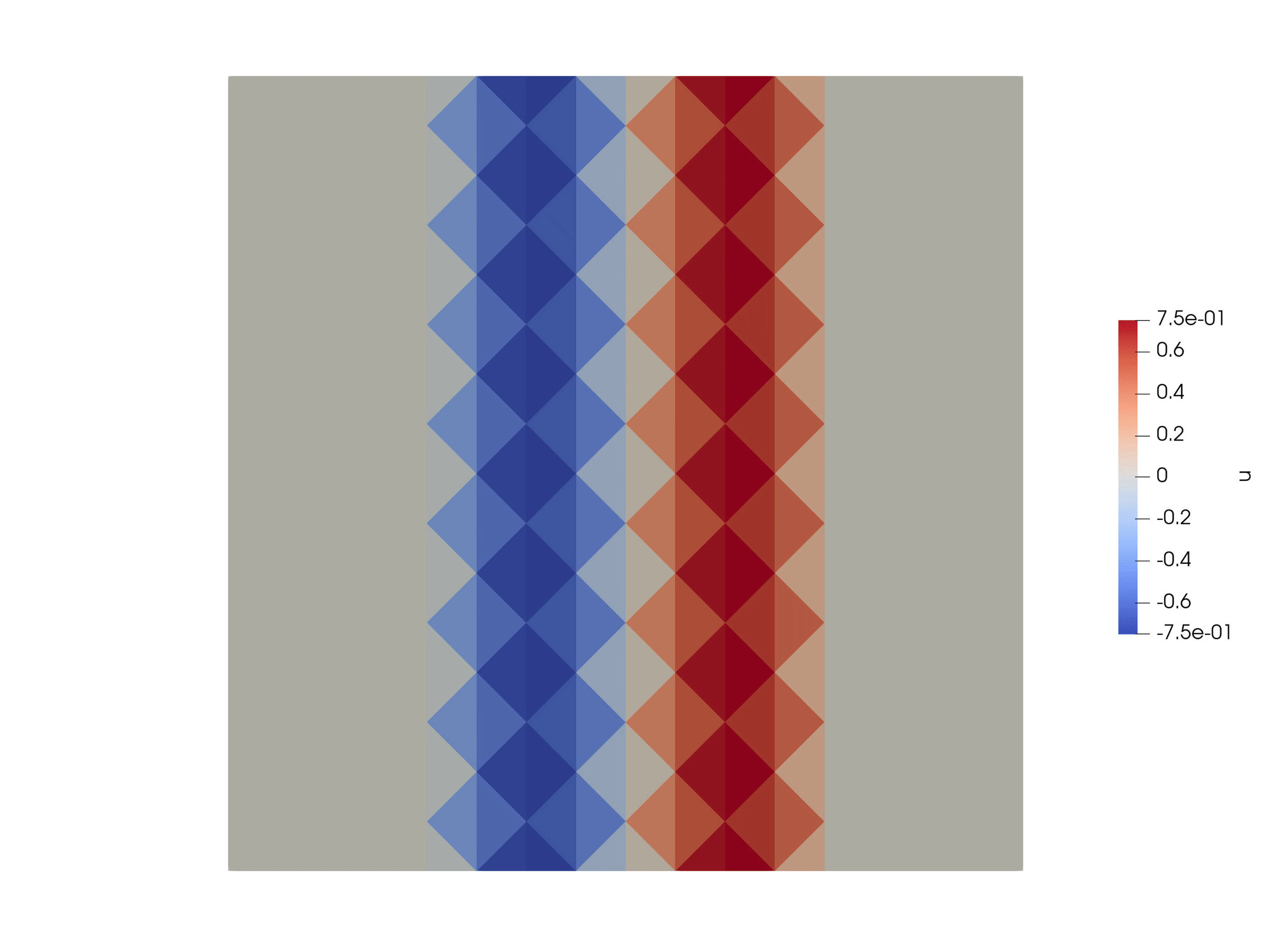
Fig. 2 Travelling wave example, wave speed is higher in the middle than at the top and bottom.#
The Travelling wave can be configured in the parameter file (in the IniCondition section):
origin = 0 0 0describes a point on the (initially) planar wave.kVec = 6.283 0 0is the wave vector. The wavelength can be computed as \(\lambda = 2\pi / \|k\|\). In this case it travels in the direction of the x-axis, the wave length is \(1 m\).ampField = 2 0 0 0 0 0 0 1 0describes the amplitudes of the different wave modes. We can impose aPwave and twoSwaves with different polarizations travelling either in the same direction (+) or in the opposite direction (-) of \(k\). Note: there are three non propagating modes (N). The entries of \(k\) are-P -S -S N N N +S +S +P. In this example, we impose a P wave travelling in the opposite direction as \(k\) with relative amplitude \(2\) and an S wave travelling towards the same direction as \(k\) with relative amplitude \(1\).
Scholte (Scholte)#
A Scholte wave to test elastic-acoustic coupling
Snell (Snell)#
Snells law to test elastic-acoustic coupling
Ocean (Ocean)#
An uncoupled ocean test case for acoustic equations
How to implement a new hard-coded initial condition?#
Alternatively, you can implement a new initial condition in the code itself.
For that, extend the class
seissol::physics::Initalfield
and implement the method
void evaluate(  double time,
                const std::array<double, 3>* points,
                std::size_t count,
                const CellMaterialData& materialData,
                yateto::DenseTensorView<2,real,unsigned>& dofsQP ) const;
Here dofsQP(i,j) is the value of the \(j^\text{th}\) quantity at the points[i].
Furthermore, you will also need to add the new initial condition to the paraemter file parser
in src/Initializer/Parameters/InitializationParameters.cpp and the initial condition initialization
under src/Initializer/InitProcedure/InitSideConditions.cpp as well.