SCEC TPV29

TPV 29 contains a vertical, right-lateral fault with rough fault interface (Fig. 32). The fault surface has 3D stochastic geometrical roughness (blue and red colors). In TPV 29, the surrounding rocks respond elastically.

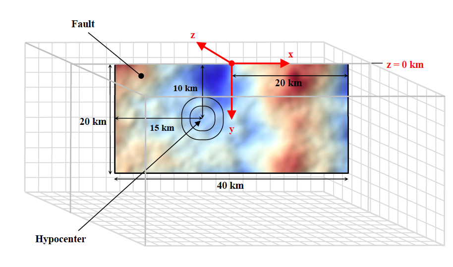
Fig. 32 Diagram of TPV 29. The fault is 40 km long along the strike. There is a circular nucleation zone on the right-lateral fault surface. The fault surface has 3D stochastic geometrical roughness (blue and red colors). The hypocenter is located 15 km from the left edge of the fault, at a depth of 10 km.

Geometry

The roughed fault interface model is generated with Gmsh is complicated than planar faults in previous sections. There are 5 steps to generate the model.

1.Download fault topography data from SCEC. There are 2001 nodes

along the strike and 1201 nodes along the downdip. The node files should contain:

Line 1: nx, ny
Line 2 to nx: positions of nodes along the strike (in meters)
Line nx+3 to ny+nx+3: positions of nodes along the downdip (in meters)
Line to the end: fault topography of each nodes (nx\*ny, in meters)

Using generate_mytopo_tpv29.py to create the topography data.

2.Make a model with plane fault as Fig. 33. The Gmsh tpv29.geo file can be found at SeisSol/Examples.

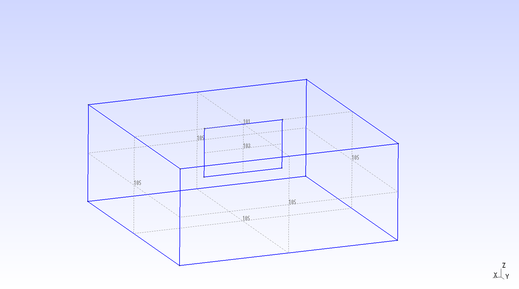
Fig. 33 Diagram showing the geometry of TPV 29. The center of nucleation is at (-8, 0, -10) km on the main fault.

3.Use gmsh_plane2topo.f90 and interpol_topo.in* to shift the planar fault according to positions given in mytopo_tpv29.

$ ./gmsh_plane2topo interpol_topo.in

This will generate a step1_modified.msh file which containing rough fault surface.

4.Make a new step2.geo file that contains the new rough fault and mesh following general Gmsh process.

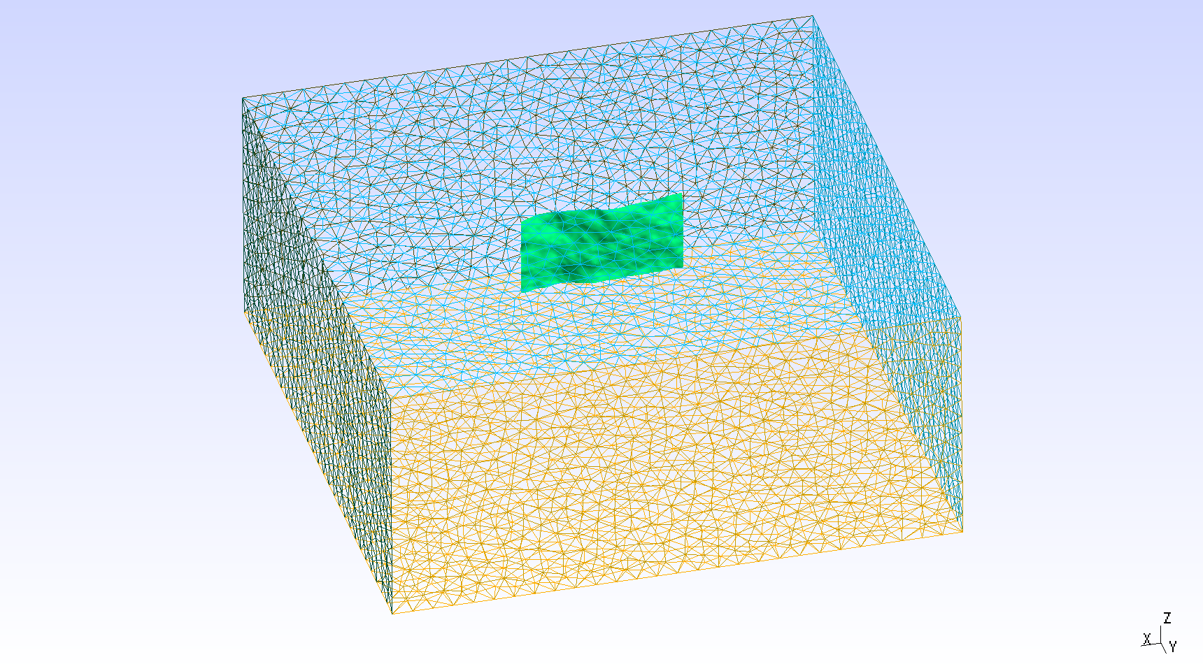
Fig. 34 Diagram showing the geometry of TPV 29. The center of nucleation is at (-8, 0, -10) km on the main fault.

5. Generate MSH mesh with the command line:

& gmsh tpv29_step2.geo -3 -optimize_netgen -o tpv29_step2.msh

The option -optimize_netgen is necessary for optimizing meshing with good quality.

6.Then convert the .msh file to the PUML format; in the same way as it is shown for TPV5:

::

$ pumgen -m msh2 tpv29_step2.msh tpv29

The mesh can be created by using the bash script SeisSol/Examples.

Here we show a fully opensource workflow which allows generating a mesh accounting for tpv29 rough fault geometry. This yields a mesh that does not properly account for the intersection between fault and the free-surface. We note that it is here not an important issue, as the tpv29 benchmark does not feature surface rupturing. Another drawback of this workflow is that the rate of mesh size coarsening is not easy parametrizable. A more straightforward and accurate way to generate a mesh would be to use simModeler.

Material parameters

In TPV29, the entire model volume is a linear elastic material, with the following parameters listed in Table 7.

Table 7 Material parameters for TPV29.

Parameter	Description	Value	Unit
\(\rho\)	density	2670	\(kg/m^{3}\)
\(\lambda\)	Lame’s first parameter	3.2044e10	Pa
\(\mu\)	shear module	3.2038e10	Pa
\(h_{edge}\)	element edge length	200	m
\(V_p\)	P wave velocity	6000	m/s
\(V_s\)	S wave velocity	3464	m/s

Initial stress

The initial stress are listed in Table 8.

Table 8 Fault parameters for TPV29.

Parameter	Description	Value	Unit
mu_s	static friction coefficient	0.12
mu_d	dynamic friction coefficient	0.18
d_c	critical distance	0.30	m
s_zz	\(\sigma_{zz}\)	-2670*9.8*depth	Pa
Pf	fluid pressure	1000*9.8*depth	Pa
s_xz,s_yz	\(\sigma_{xz}, \sigma_{yz}\)	0	Pa
s_yy		\(\Omega * b33*(\sigma_{zz} + P_f) - P_f\)	Pa
s_xx		\(\Omega * b11*(\sigma_{zz} + P_f) - P_f\)	Pa
s_xy		\(\Omega * b13*(\sigma_{zz} + P_f)\)	Pa

Table: Table of initial stress in TPV 29. \(b11, b33,b13\) are 1.025837, 0.974162, −0.158649, respectively.

Note that the effective stress tensor is :

\[\begin{split}\bar{\sigma}_{effective}= \begin{bmatrix} &\sigma_{xx} + P_f , & \sigma_{xy} ,& \sigma_{xz} \\ &\sigma_{xy}, &\sigma_{yy} +P_f , &\sigma_{yz} \\ &\sigma_{xz} ,&\sigma_{yz} , &\sigma_{zz} +P_f \end{bmatrix}\end{split}\]

where \(\Omega\) is defined as:

\[\begin{split}\Omega = \left\{ \begin{array}{lr} &1, depth \leq 17000 m \\ & (22000 - depth)/5000 m, 17000 < depth < 22000 m \\ & 0, depth \geq 22000 m\\ \end{array} \right.\end{split}\]

Nucleation parameters

TPV29 uses a similar strategy for dynamic rupture nucleation.

\[\begin{split}T = \left\{ \begin{array}{lr} & \frac{r}{0.7Vr} + \frac{0.081*r_{crit} }{0.7Vr} (\frac{1}{1-(r/r_{crit})^2} - 1), r \leq r_{crit} \\ & 1E+09, r > r_{crit}\\ \end{array} \right.\end{split}\]

The cohesion zone is defined as :

\[\begin{split}C_0 = \left\{ \begin{array}{lr} & 0.4 MPa + 0.000675 MPa * (4000- depth), depth < 4000 m \\ & 0.4 MPa, depth \geq 4000 m\\ \end{array} \right.\end{split}\]

The friction parameters on the fault are listed in Table 9.

Table 9 Table of friction parameters in TPV 29.

Parameter	Description	Value	Unit
mu_s	static friction coefficient	0.12
mu_d	dynamic friction coefficient	0.18
d_c	critical distance	0.30	m
t_0	forced rupture delay time	0.5	s

Results

The earthquake rupture is artificially nucleated in a circular zone on the fault surface.

Fig. 35 Snapshot of slip rate along the strike at T=3 s in TPV 29. The fault has a rough surface.