SCEC TPV34#
The TPV34 benchmark features a right-lateral, planar, vertical, strike-slip fault set in a half-space. The velocity structure is the actual 3D velocity structure surrounding the Imperial Fault, as given by the SCEC Community Velocity Model CVM-H.
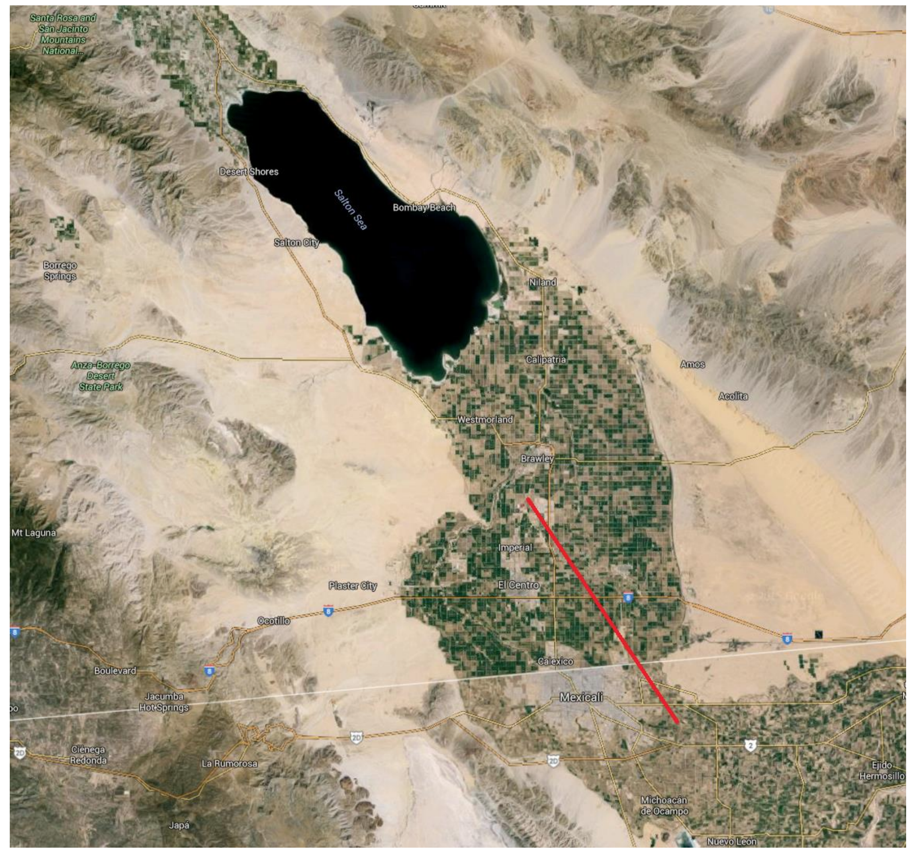
Fig. 36 The Imperial Fault. The red line marks the Imperial Fault. It straddles the California-Mexico border, south of the Salton Sea. The Imperial Fault is approximately 45 km long and 15 km deep, with a nearly vertical dip angle ranging from 81 to 90 degrees according to the SCEC Community Fault Model CFM-4.#
Geometry#
The model volume is a half-space. The fault is a vertical, planar, strike-slip fault. The fault reaches the Earth’s surface. Rupture is allowed within a rectangular area measuring 30000 m along-strike and 15000 m down-dip.
There is a circular nucleation zone on the fault surface. The hypocenter is located 15 km from the left edge of the fault, at a depth of 7.5 km.
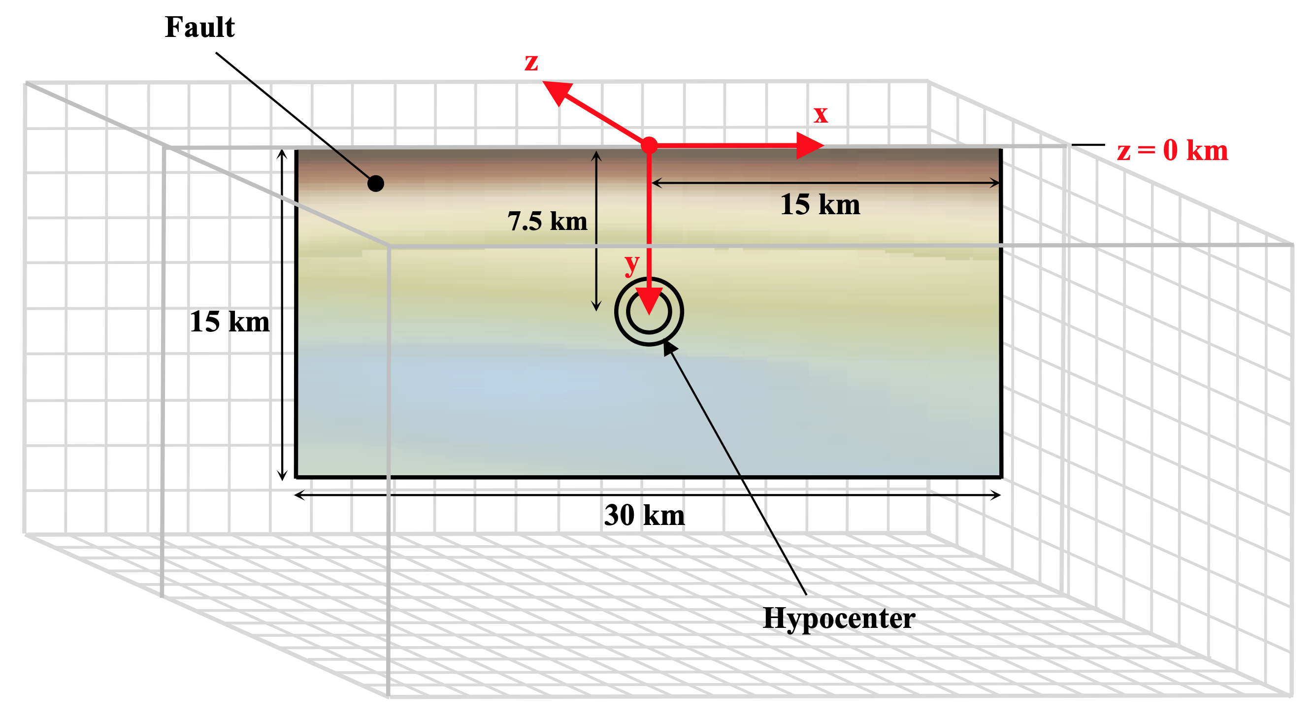
Fig. 37 TPV34 overview.#
The geometry is generated with Gmsh. All the files that are needed for the simulation are provided at SeisSol/Examples.
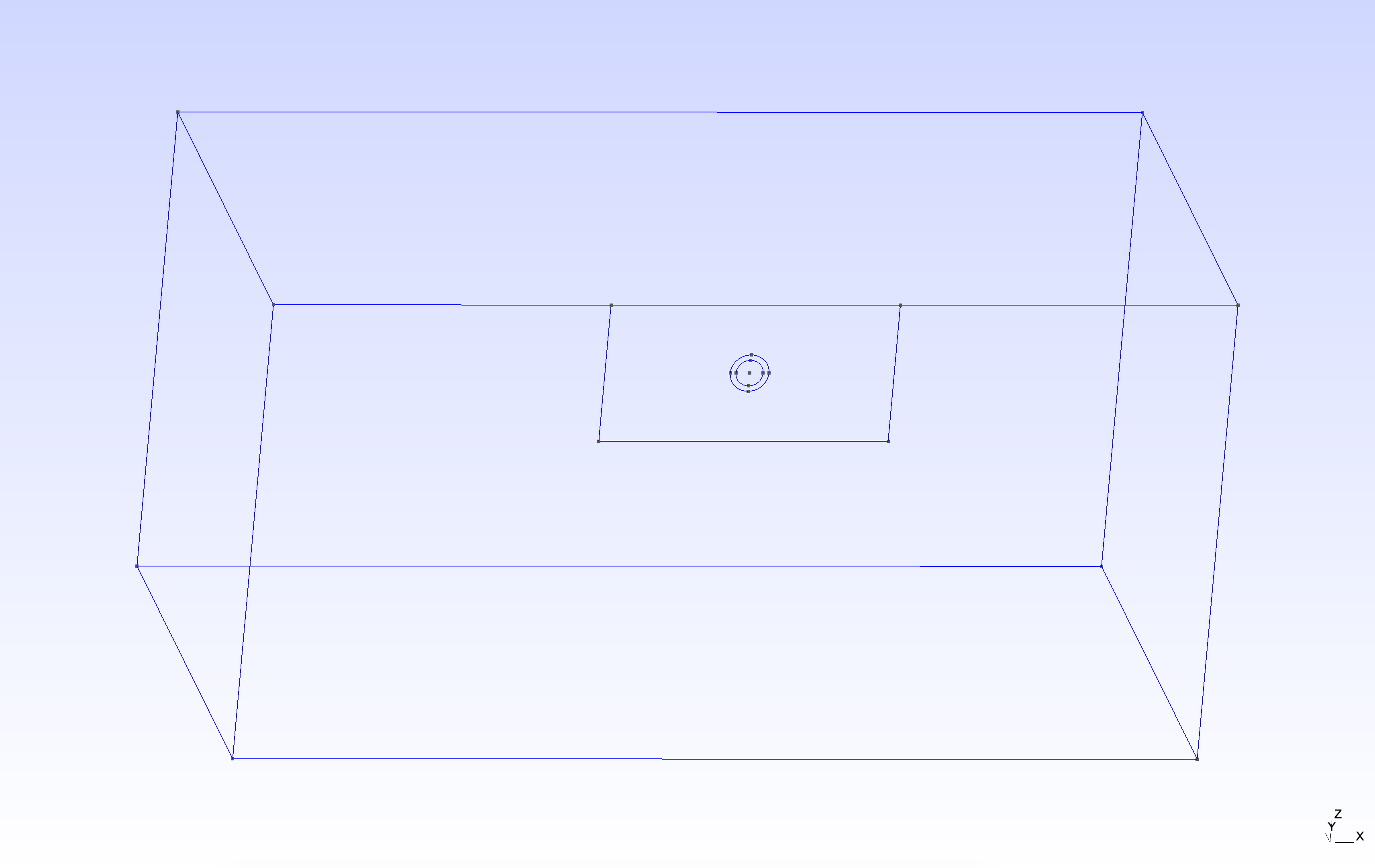
Fig. 38 Modeled TPV34 fault in Gmsh.#
Material#
To obtain the velocity structure for TPV34, we need to install and run the SCEC Community Velocity Model software distribution CVM-H. For TPV34, we are using CVM-H version 15.1.0 and we use ASAGI to map the material properties variations onto the mesh. Detailed explanations are provided at SeisSol/Examples. We generate 2 netcdf files of different spatial resolution to map more finely the 3D material properties close to the fault. The domain of validity of each netcdf files read by ASAGI is defined by the yaml tpv34_material.yaml file:
[rho, mu, lambda]: !IdentityMap
  components:
    # apply a finer CVM-H data inside the refinement zone
    - !AxisAlignedCuboidalDomainFilter
      limits:
        x: [-25000.0, 25000.0]
        y: [-25000.0, 25000.0]
        z: [-15000.0, 0.0]
      components: !ASAGI
        file: tpv34_rhomulambda-inner.nc
        parameters: [rho, mu, lambda]
        var: data
    # apply a coarser CVM-H data outside the refinement zone
    - !ASAGI
        file: tpv34_rhomulambda-outer.nc
        parameters: [rho, mu, lambda]
        var: data
Parameters#
TPV34 uses a linear slip weakening law on the fault. The parameters are listed in Table below.
Parameter |
inside the nucleation zone |
Value |
Unit |
|---|---|---|---|
mu_s |
static friction coefficient |
0.58 |
|
mu_d |
dynamic friction coefficient |
0.45 |
|
d_c |
critical distance |
0.18 |
m |
The cohesion is 1.02 MPa at the earth’s surface. It is 0 MPa at depths greater than 2400 m, and is linearly tapered in the uppermost 2400 m. The spatial dependence of the cohesion is straightforwardly mapped using Easi.
[mu_d, mu_s, d_c]: !ConstantMap
  map:
    mu_d: 0.45
    mu_s: 0.58
    d_c: 0.18
[cohesion]: !FunctionMap
  map:
    cohesion: |
      return -425.0*max(z+2400.0,0.0);
Initial stress#
The initial shear stress on the fault is pure right-lateral.
The initial shear stress is \(\tau_0\) = (30 MPa)(\(\mu_x\))
The initial normal stress on the fault is \(\sigma_0\) = (60 MPa)(\(\mu_x\)).
In above formulas, we define \(\mu_x = \mu / \mu_0\), where \(\mu\) is shear modulus and \(\mu_0\) = 32.03812032 GPa.
[s_xx, s_yy, s_zz, s_xy, s_yz, s_xz]: !EvalModel
  parameters: [radius,mux]
  model: !Switch
    [mux]: !AffineMap
      matrix:
        x: [1.0,0.0,0.0]
        z: [0.0,0.0,1.0]
      translation:
        x: 0.0
        z: 0.0
      components: !ASAGI
        file: tpv34_mux-fault.nc
        parameters: [mux]
        var: data
    [radius]: !FunctionMap
      map:
        radius: |
          xHypo =     0.0;
          zHypo = -7500.0;
          return sqrt(((x+xHypo)*(x+xHypo))+((z-zHypo)*(z-zHypo)));
  components: !FunctionMap
    map:
      s_xx:     return -60000000.0*mux;
      s_yy:     return -60000000.0*mux;
      s_zz:     return 0.0;
      s_xy: |
        pi = 4.0 * atan (1.0);
        s_xy0 = 30000000.0*mux;
        s_xy1 = 0.0;
        if (radius<=1400.0) {
          s_xy1 = 4950000.0*mux;
        } else {
          if (radius<=2000.0) {
            s_xy1 = 2475000.0*(1.0+cos(pi*(radius-1400.0)/600.0))*mux;
          }
        }
        return s_xy0 + s_xy1;
      s_yz:     return 0.0;
      s_xz:     return 0.0;
Results#
All examples here can be visualized in Paraview. The output folder contains a series of files for fault dynamic rupture (hdf5 and .xdmf), wavefield (hdf5 and .xdmf), on-fault receiver (.dat) and off-fault receivers (.dat). The fault dynamic rupture and wavefield files can be loaded in Paraview. For example, open Paraview and then go through File > import > ‘prefix’-fault.xdmf.
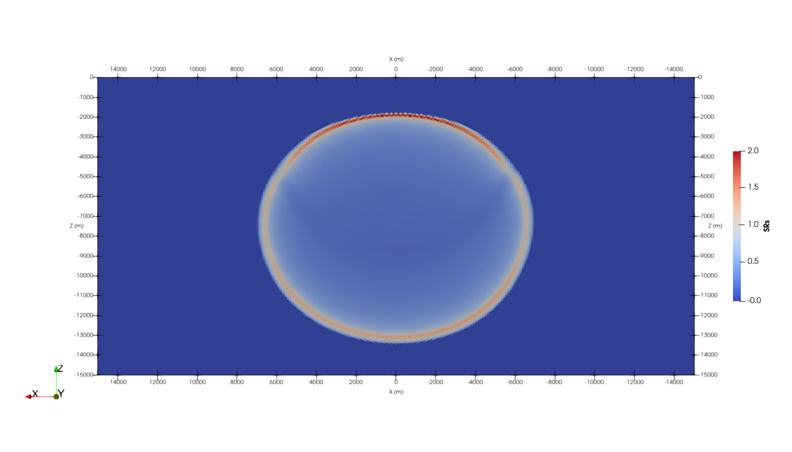
Fig. 39 Fault slip rate in the along-strike direction (SRs) at a rupture time of 3 seconds in TPV34, visualized using Paraview.#